
About This Note
This Note is constructed into multiple parts, each based on the content of a big subject or field. In each part are topics that were sorted in ascending difficulty based on Luke's personal experience, not necessarily based on the actual comprehension difficulty.
When reading about a topic, it is expected that you will start to search about the terminologies as well as the concepts that were mentioned that you did not understand. A good place to begin looking up is in this guide itself before going to the internet. Despite there being topics that are "harder" than other topics, it does not mean that learning the latter is the requirement for the "more difficult" topics.
This Note was written in a way to provide intuition to difficult topics, giving a different perspective to digest a concept. On other topics, this Note acts as a cheat sheet for a quick review before tests. Whatever the case might be, I hope you find this Note somewhat helpful on the path that you choose. It is recommended that you follow through on a topic to the end, as most of the time topics are structured in a way that does not repeat the mentioned notices more than once.
A lot of times, the topics are cross-disciplined and are useful in multiple fields, making sorting them into one particular part difficult. If that is the case, the topic will be put in a Part that is the most popular to be associated with that topic, then other cross-disciplined fields will be indicated in a bracket on the title of that topic. Therefore, if you did not find a topic you want to see in a part, maybe other parts will contain the concept you want to understand.
An explanation of the reason why the parts were ordered the way it is: the author believed that math is the foundation of sciences, so it was put in the beginning. Biology will be followed after it because it is the science that is (mostly) visible to human application — it is the first machine being built based on the other science. At a lower level, chemistry will explain the interaction between substances that make up the organs and show how to build those living machines. Physics was put last but not least because physics itself describes the rules that others must follow. The order itself is less of something academic but more of the personal belief of the author.
The Note of Science Topics by Luke NK is free and unlicensed. The author simply suggests the astute reader share this with anybody who needs a different perspective to look at the topics. Knowledge is best used when everybody knows it.
Math
Logic and Proofs
Logic is very easy to understand. If it is hard for you, you have a bigger problem that this chapter cannot solve. However, to save time, mathematicians created multiple notations to make their lives easier (and our lives a bit harder). This chapter is an attempt to quickly summarize those notations and acts as a reference sheet whenever you see strange logic notations.
Symbols and notations
Propositions are statements that could be either true or false. We use $T$ or $F$ to indicate true or false.
A proposition can be negated, which gives the opposite of the proposition. The negation of $p$ is:
The conjunction operator will return true if both propositions $p$ and $q$ are true; it is similar to an “and” statement.
Disjunction is similar to an “or” statement where it only requires either one statement to be true.
Exclusive or (XOR) will return true if either statement is true, but not both.
It is similar to $(p \lor q)\land\neg(p \land q)$.
Implication expresses that one thing will result in another (“if $p$ then $q$”):
$p$ is called the antecedent, premise, or hypothesis; $q$ is called the conclusion or consequence because it is the result of $p$. Moreover, noted that the whole statement itself can still generate $T$ or $F$ values. If we have a statement “If the store is open today ($p$), then Luka will go ($q$)”. Consider the truth table, we have:
- If the store opens, then Luka will go, making $p \rightarrow q$ true.
- If the store opens but Luka does not go, then apparently Luka’s action does not depend on the store being opened.
- If the stores do not open but Luka still goes, the statement $p \rightarrow q$ is still true because it does not say anything about the store being closed.
- If the store closes and Luka stays at home, the statement is still true for a similar reason.
A bi-conditional statement is similar to the statement “if and only if”, that is when both propositions support each other. This is similar to the equal sign, so even if both propositions are false, the bi-conditional statements still hold (because $F=F$)
The difference is that bi-conditional implies that both $p$ and $q$ are similar to each other; that is, they are either both true or both false for $p \leftrightarrow q$ is true.
Equivalent are propositions that are the same. There are two ways to write it and you will usually see the latter in algebra:
A predicate is a statement with variables, written with a capital letter and a variable listed as arguments:
Predicate is the founding block of functions — that is why the function notation is similar to this. Once the variables have values, it is a proposition with a determined true or false result.
The universal quantifier is used to denote sentences with words like “all” or “every”:
Essentially that statement allowed us to plug every possible $x$ into our predicate $P(x)$.
The existential quantifier is used to denote sentences with words like “some”. It implies the fact that there are at least some variables that make the predicate $P$ hold.
Informally, $\forall$ is just a bunch of $\land$s and $\exists$ is just a bunch of $\lor$s.
Noted that for nested quantifiers, the order does matter: \[ \forall x \exists y (x+y=0) \qquad \exists x \forall y (x+y=0) \] The first one is: “For all $x$, there exists $y$ that makes the predicate true”. The second one is saying “There is some $x$ that when you select any $y$, the value $x+y=0$”.
Therefore symbol is:
At the end of a proof, Q.E.D. is used to show that the proof is completed.
Logic proof
Inference is when you prove something is true by proving that everything we know is true is equivalent to $q$, therefore $q$ must be true.
If $p$ leads to $q$ and $p$ is true, then it will lead to $q$ is true.
A few logic terms:
- Proof: a valid argument based on theorems and what is known to be true.
- Conjecture: a statement that you think is true and will be proven with your proof
- Theorem: a statement that has been shown to be true
- Premise: a condition or a requirement for something to be true
- Lemma: a small theorem that we need to get to the proof we are interested in
- Corollary: a small theorem that is the result of the more important theorem
Disproving conjecture is a proving method that applies to theorems with $\forall xP(x)$, where you can simply find a single $x$ that dissatisfies $P(x)$.
Direct proof assumes that $p$ is true, then follows implications to show that $q$ is true. This is similar to how you do algebra where you make multiple $=$ lines to get to your answer. To be more exact, it is algebra that gets this idea from logic. This is the application of hypothetical syllogism:
Proof by induction is simply proving that $P(n)$ is true for $1$, then proving that $\forall n=k\leq1$, it is still true with $n=k+1$.
Proof by contraposition utilizes this rule:
In simple terms, proof by contraposition simply proves that if $q$ is wrong then $p$ must be wrong too, and then we prove that because $p$ is right then $q$ is right.
The existence proof is useful for statements like $\exists xP(x)$. Just simply find one $x$ that satisfies $x$ and you are done. Disproving such a statement is harder because then you must prove that $\forall x$, $P(x)$ is false.
Sets
Because sets are fairly simple to understand, this chapter will act more as a quick reference sheet.
Basic
Sets are written with curly braces with its elements separated by a comma:
Order does not matter and duplicates do not count. If there are two similar elements then they are treated as one.
Element-of symbol is written as:
Two sets are equal if they contain the same elements.
“$A=B$ if and only if for all $x$ in $A$, there exists a similar $x$ in $B$”.
A set can contain another set:
A set’s cardinality is the number of distinct elements. We only count the number of objects in the set we are evaluating (only counting the number of elements at the top level).
Instead of listing everything (maybe even with dots $\dots$), you can describe the elements of a set with set builder notation:
In that notation, $n$ was defined as a variable that will go in the set; the condition for $n$ was put after the vertical line.
An empty set has a special notation:
Any non-empty set will have $\emptyset$ as its subset:
A subset can be noted like this:
Note that there is a difference between a subset and being an element. A proper subset is a subset that is not identical. The underline below the subset symbol is similar to the equal sign in $\leq$ sign.
A power set is a set containing all of a set’s subsets:
Notice that the power set contains the set $S$ itself (as the definition is not a proper subset) and an empty set $\emptyset$. The cardinality of a power set is $|P(S)| = 2^{|S|}$.
Cartesian product is all possible ways to take things from two sets. The Cartesian product of sets $A$ and $B$ is the set of all ordered pairs of values from $A$ and $B$.
Cartesian product is not commutative:
Set operation
The union of two sets contains all elements from both of those sets. It is the set of all elements from both sets:
The intersection of two sets is the set containing elements that appear on both sets:
Note that the symbols are similar to the “and” logic operator ($\land$).
The difference between two sets is the set of values in one but not the other, similar to subtraction:
The difference does not have commutative property.
Similar to sigma notation, we can describe a large number of sets with:
[Science] Significant Figures, Rounding, and Scientific Notation
Significant figures (digits), usually denoted with “SF” in Canada, is considered to be the level of precision of a number. The amount of significant figures you have implies the accuracy of your number. The rules are very easy to follow:
- All leading zeros are not significant
- If there is a decimal point, all trailing zeros are significant
- Digits between the first and the last non-zero digit are significant
- If a digit is significant but the rules above do not cover, you can underline it
Remember, the second point only counts trailing zeros, which are zeros after a non-zero digit, regardless of where the decimal point is.
We can add “plus/minus” ($\pm$) to further show our level of accuracy.
Rounding is simply reducing the number of significant figures. Here is an additional rule you might not know about rounding 5: you should round it to make the last digit even. This ensures that the ups and downs will cancel out each other over a long chain of calculations.
Scientific notation
Scientific notation is a way to deal with very big or very small numbers. There are two parts in a scientific notation: the mantissa $m$ (decimal portion) and the exponent $n$ (ordinate):
A good way to think of the exponent $n$ is in terms of how you move the decimal point in the mantissa $m$. If $n$ is positive, move the decimal point to the right $n$ times (which is $\times10^n$), and vice versa for a negative power.
A constraint for the mantissa to prevent people from writing the number too hard to read is it must be between 1 and less than 10 ($1 ≤ |m| < 10$). If you have $0.6$, simply move the decimal to the right and subtract the exponent by $1$, which gives you $6\times10^{-1}$. The mantissa can be also negative ($-1.3\times10^1$ for example). When dealing with negative scientific notation, just treat it like a normal notation and do not confuse between negative mantissa and negative exponent.
Ten raised by zero equals 1, useful to represent numbers with the right mantissa but does not hint at the fact that it is in scientific notation:
To convert a number to scientific notation, simply move the decimal point until it satisfies the mantissa’s requirement. To remember which sign to put for the exponent: if you moved the decimal point to the left (making the mantissa smaller), then you need to multiply it by a factor of $10$ to make it the same as the original number. Ask yourself: do I need the exponent to be bigger or smaller to make the mantissa equal the original number?
Scientific notation is helpful when counting significant figures because now all of the digits that appear in the mantissa are significant.
To add/subtract numbers in scientific notation, make the exponent the same and simply deal with the mantissa, then readjust the result to proper scientific notation by moving the decimal. The answer should be rounded to the least number of decimal places.
\[\begin{aligned}
& 3.0 \times 10^2 + 6.4 \times 10^3 \qquad 300 + 6400 \\
=& 3.0 \times 10^2 + 64 \times 10^2 \qquad \text{least number of decimal places is }0 \\
=& (3.0 + 64) \times 10^2 \\
=& 67.0 \times 10^2 \qquad \text{round the number, return the mantissa to scientific notation} \\
=& 6.7 \times 10^3
\end{aligned}\]
To multiply/divide, you also multiply/divide the mantissa by themselves first, then multiply/divide the exponents by using an exponent rule $10^n\cdot10^m=10^{n+m}$. This was hidden behind the fact that multiplication is commutative. The answer should have the same significant figures as the number with the least significant figures.
\[\begin{aligned}
& (4.1\times10^6)\times(3.110\times10^8) \qquad\text{2SF} \times\text{4SF} \\
=& (4.1\times3.110)\times10^{6+8} \\
=& 12.751\times10^{14} \qquad \text{round to 2SF and shift decimal point} \\
=& 1.2\times10^{15}
\end{aligned}\]
Complex Numbers
Introduction
The definition of a complex number:
We define the real part of $z$ as $Re(z)=a$ and the imagined part $Im(z)=b$. Furthermore, we define the conjugate of a complex number as $z^*$ (z star):
Because $b=0$ for real numbers, the conjugate of a real number is itself.
Visual intuition
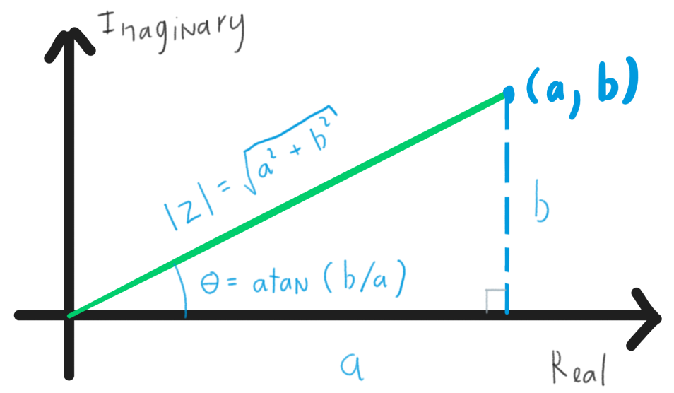
As a way to draw it on a standard two-axis graph similar to , you can put the horizontal axis (x-axis) as $a$ and the vertical axis as $b$ to represent the imaginary part of a complex number. This works better if you also recall that we were taught real numbers on a left-right number line.
With this intuition, a number will have a certain “distance” away from the origin. When finding the conjugate of a complex number, you are essentially flipping the vertical axis. If you pay close attention to , you can see that it closely resembles the standard graph form $y=mx+b$.
Identities
The norm of a complex number, which visually is the length of the vector from the origin to $z$ on a plane, is denoted as $\mid z \mid$:
Another fundamental equation is the norm squared which is the direct result of the norm itself:
The proof for these identities can be worked backward. Furthermore, the norm squared is used to calculate the probability of a state in quantum physics, something you should keep at the back of your mind if you want to pursue that field.
From the visual intuition we established above, a complex number represented on a unit circle (the norm is equal to 1) can also be written with trigonometric functions:
Complex number calculations
Adding and subtracting two complex numbers is just simply doing every part individually:
Remember to pay close attention to the negative sign at the beginning of the second term when subtracting.
Multiplying two complex numbers is simply using FOIL (multiplying terms together). Another extended version of FOIL that requires a bit of memorization is:
A fascinating fact is when you multiply a complex number by $i$, the result is another complex number vector that is $90^\circ$ (or $\pi/2$) counterclockwise.
Dividing is a bit of work. You start with a fraction, then multiply the first fraction by another fraction with both the numerator and the denominator as the conjugate of the first fraction’s denominator (making the second fraction equal to 1). Here is an example:
\[\begin{aligned}
&\frac{2 + 3i}{4 - 5i} \\
=& \frac{2+3i}{4-5i} \cdot \frac{4+5i}{4+5i} \\
=& \frac{(2 + 3i)(4 + 5i)}{4^2 + 5^2} \qquad (a + bi)(a - bi) = a^2 + b^2 \\
=& \frac{8 + 10i + 12i - 15}{41} \\
=& \frac{-7 + 22i}{41}
= -\frac{7}{41} + \frac{22}{41}i
\end{aligned}\]
Polar form
The polar form provides you with another “description” of the very same point on the plane. Instead of identifying a point on the plane using the axes, we use the distance from the origin and the angle from the positive x-axis instead. Notation-wise, $r$ is the radius from the origin (the distance) and $\theta$ is the angle from the positive x-axis. We can do a conversion from Cartesian to Polar:
From Polar to Cartesian, we can calculate the $x$ and $y$ separately using $\cos$ and $sin$:
A common way to write a complex number in Polar form is by getting the unit vector multiplied by the radius:
Multiplying in Polar form
The polar form provides intuition to complex multiplication problems. When multiplying two complex numbers together, the magnitudes get multiplied and the angles get added.
This also explains why multiplying with $i$ with get a complex number that is perpendicular to the start vector. $i$ simply added $90^\circ$ to the angle and kept the radius the same.
From , we can yield the general formula when raising a complex number by an exponent, called De Moivre’s formula:
\[ \Rightarrow r_{result} = r^n \qquad \theta_{result} = n \times \theta \]
Permutation and Combination
The difference between permutation and combination is in the order. Permutation is an ordered combination or in other words, a combination does not concern the order.
Order does not matter here means that a 123 string is the same as a 213 string.
When approaching statistical problems relating to permutation or combination, the basic approach should be calculating every individual part that you can count, then dividing to remove the over-count or multiplying to compensate for the under-count.
Permutation
Permutations with repetition
When $n$ is the number of elements and $r$ is how many times we can select the elements, the number of possible permutations we can have is:
For example, every time we roll a dice, there are 6 possible results (faces). If we roll it once again, now there are 6 results for every previous roll’s result $6\times6$. If we ask how many permutations there are after 3 rolls of dice, the result is $6^3=216$ permutations. Every time we roll the dice, there is the possibility that a face will repeat (hence repetition is allowed).
Permutations without repetition
Four people were tasked to line up in a straight line, how many possible line arrangements can we get? There are four possible people to stand at the first position; for every selection, there will now be three possible candidates to stand at the second position, and so on… A person cannot appear twice in a line (not a quantum physics topic) so our choice gets reduced each time.
The formula is:
and despite being unrelated to statistics, this is a property of factorial:
Continuing with the example above, what if we want to find how many possible line arrangements with only two people? In this question, we are “cutting short” our factorial formula because there are no more selections after the second person. To do that, we cancel the spare part by dividing it by itself:
$n \ge r$ as you cannot have a collection longer than the number of elements you have. In this formula, the second notation was commonly seen on calculators, while the third notation is common in Vietnam (with $P$ being replaced with $A$).
Combination
The most common version you will need is combinations without repetition, so treat the combination with repetition as some extra reading.
Combinations without repetition (regular combination)
We want to pick two people from four people. We do not care about the order we pick but rather how many people we pick. Say if we picked Luke and Luna:
- If the order does matter: there are two possibilities: Luke first or Luna first.
- If the order does not matter: only one possibility: Luke and Luna.
So as you can see, permutations have twice the possibilities. You can calculate how many possibilities permutation has more than combination by using permutation on the subset itself (in this case, the set contains Luke and Luna): \[ P(r, r) = r! \] Now we simply divide our permutation formula with this spare part to get our combination formula:
You still need to keep in mind the fact that if an item was selected, it cannot be selected again in this non-repetition version (our example selection cannot have two Lukes or Luke will have to do a job twice).
Combination with repetition
This is a combination without repetition, but we plug in a different number to achieve our goal. Unfortunately, it is quite difficult to explain the algebraic proof so instead, this section will based on the visual intuition of one particular example.
We want to buy six tea bags, with three different flavours: (A) aloe vera tea, (B) black tea, or (C) chai tea. In this case, there are two important factors:
- Repetition is allowed: we can pick a tea flavour more than once
- The order does not matter: we only care about how many we have picked
Because order does not matter, we will list our teas in the same order: A then B then C. Next, we will add a separator between the teas. Here is what our diagram will look like:
\[\begin{bmatrix}
-&-&-&|&-&-&|&- \\
|&-&-&-&|&-&-&- \\
|&-&-&-&-&-&-&| \\
|&|&-&-&-&-&-&-
\end{bmatrix}\]
There are still six dashes representing our six allowed selections, while the two separators simply indicate that we are moving between the types of tea. In the second example, you can see that we did not select A but only B and C. The third example only shows that there was only B that was selected; similar to C in the fourth example
With that diagram, the answer broke down to how many ways we can put down these two dividers. We have $n=3$ teas which means we have $n-1$ separators; There are $r+n-1$ spaces including the items and the separators to insert the divisors:
This calls: select space to insert $n-1$ separators. Now you may ask why it is not simply $r-1$ (the space between the items only). It is because we always have the possibility that two separators are standing next to each other — such a case would not be covered by the $r-1$ where there is no “space” for the separators to stand next to each other.
The $n-1$ on the denominator gets from $n+r-1-r$ being cancelled, therefore we have the official combination with repetition formula:
The first hint to realize that you are dealing with combinations without repetition is in the fact that $n < r$. In our example, we had more positions to fill than the items we had, so we must repeat some. Notice that in this case, $n$ and $r$ “swapped” places for each other compared to other formulas; what we plugged in our original combination formula is still the same though.
Solving problems
How many ways we can rearrange the word “Canada”? This question cares about the order, so the first step is to get the basic permutation with the factorial formula $6!=720$. However, notice that there are three different “a” inside that word, so we need to “remove” that over-count. We do that by dividing our over-count by the number of possible arrangements of the three “a” characters: \[ \frac{6!}{3!} = 240 \]
Most of the time when solving statistical problems, it is about you determining how much you have over-counted, then removing that spare part by dividing.
From 1, 2, 3, and 4, how many 3-digit numbers (with non-repeating digits) can we get that are smaller than 320? The first digit of our number will need to be either 1 or 2 to be certain that any number selected after it will be smaller than $320$. Because this is non-repeating, after we select either 1 or 2, we only have $3$ options left for the second digit, and $2$ options for the last digit; the number of possibilities is: $2\times3\times2$. If the first digit is 3, there is only one possibility for the second digit: 1 because otherwise, the number would be larger than $320$. The final result for this route can be calculated with $1\times1\times2$ or can be counted by listing $312$ and $314$. \[ (2\times3\times2) + (1\times1\times2) = 14 \]
For this problem, an addition was used because we counted by part instead of under-counting every possibility. One thing to highlight this type of problem is when your logic route has conditional statements “if”.
In both questions, we solved not by blindly applying the permutation or combination formula but rather by starting from scratch. This is extremely useful to help you keep track of what you are counting or for problems with multiple datasets to consider.
Limit
Despite the author trying their best to explain this chapter for complete beginners, it is still expected that the reader has some basic understanding of limits. Please go read about limits somewhere first before hopping on this guide.
Approach and limit
Approach is the concept that a variable reaches closer and closer to a number. Limit is both the upper bound and the lower bound of something, like my patience for example. If we consider $x$ as the input and the value of $f(x)$ as the output, then we think limit as the bound for which the output could be given an input.
Say we have a function that spreads one butter cube into two slices of bread ($g(x)=2x$). As we get closer and closer to two cubes ($x\to2$), then the number of bread slices we can spread will approach four slices. Represent that in a mathematical term, we have: \[ \lim_{x\to2}g(x) = 4 \]
You may wonder: why I said that the limit is both the upper and the lower bound but my result only gives out one value. This is because the difference between the upper bound and the lower bound is approaching one single number. If you have two butter cubes, both the maximum and the minimum you can spread is 4. Later you will see that is not always true for certain equations.
Another interesting thing is that the limit is essentially what the value of the function is supposed to be. In our case, we evaluate that limit by simply plugging $g(2)=4$. This is the property we got from the definition of limit itself: it is the “restriction” of the y-axis (the output) as the x-axis (the input) gets closer to a value (). If x “squeeze” then it will result in $g(x)$ being squeezed to a value. This is why when solving limits, it is about arranging your function to the point where you can plug in the $x$ value to answer your limit.
The biggest takeaway from this section is: limit is what the output approaches given the input is approaching a number. Moreover, because both the upper bound and the lower bound approach a number, we can think of the limit as a value that the function is supposed to be at a given x-coordinate, even if the function is undefined at that point.
Limit from different sides
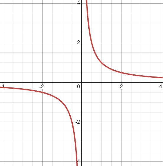
The example above “squeezes” the x-axis from both sides but what if we have an equation like ?
No matter how hard you push the x-axis from two sides together, the y-axis limit will not get smaller. If we let $x$ approach from the left side (negative side) then the limit approaches $0$; if we let $x$ approach from the positive side then the limit approaches $1$. This is the situation we mentioned earlier about the upper bound and the lower bound creating a range instead of approaching one single number. In this case, we can only state what the limit approach as $x$ approaches from either side: \[ \lim_{x\to0^-}f(x) = 0 \qquad \lim_{x\to0^+}f(x) = 1 \] Be careful: the sign denotes where we start. If the sign is negative, we approach it from the negative side and move to the positive side. I do not know why I used to mistake between those two, so that is a way to remember. Moreover, the limit of $f(x)$ as $x\to0$ does not exist.
A function’s limit only exists if the limit from both sides approaches the same number: \[ \text{If } \lim_{x\to a^-}f(x) = \lim_{x\to a^+}f(x) \text { then } \lim_{x\to a}f(x) \text{ exists} \] This leads us to the definition of continuity: if the limit of $f(x)$ at $a$ is equal to $f(x)$ then the function is continuous at $a$.
Unbound limit
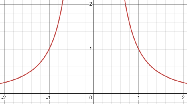
Consider the function $f(x)=1/x^2$ in , you can see that moving from both sides, the limit slowly becomes higher and higher. It seems like it is unbounded or the limit seems to reach positive infinity. \[ \lim_{x\to0} \frac{1}{x^2} = \infty \]
As you can see, both the upper limit and the lower limit still attempt to reach closer to one single value, so the limit still exists. Consider $f(x)=1/x$ in , we have the following: \[ \lim_{x\to0}\frac{1}{x} \] does not exist, but \[ \lim_{x\to0^-}\frac{1}{x} = -\infty \qquad \lim_{x\to0^+}\frac{1}{x} = +\infty \] The main limit does not exist, but the limit from either side is unbounded. The limit must exist first before continuing to check if the limit is bounded or unbounded.
Limit to infinity
Once again consider the function $f(x)=1/x^2$ as $x\to\infty$. What that means is we consider $x$ to grow to a big number and see if our y-axis merges to a number. From the graph, we can see that the value of the function is slowly reaching $0$, therefore we can state: \[ \lim_{x\to\infty} \frac{1}{x^2} = 0\]
Of course, the limit to infinity can be infinity too: \[ \lim_{x\to\infty} 2x = \infty \]
Do not be fooled! Infinity is not a variable you can move around or do mathematical operations to it. The equal sign in this case simply states that the limit is reaching a concept of extremely big numbers. We will discuss more about evaluating limit to infinity in the evaluating section. You just need to remember that the limit to infinity simply assumes that as we plug large numbers, we look if the value of the function reaches a number or not.
Solving finite limits
If we have $c$ is a constant, $a$ is the number we are trying to approach, and we definite: \[ \lim_{x\to a}f(x) = L \text{ and } \lim_{x\to a}g(x) = M \] The basic limit theorems are:
These theorems can be deducted from the concept that limit is essentially substituting $a$ into our functions, so all standard number arithmetic still works just fine.
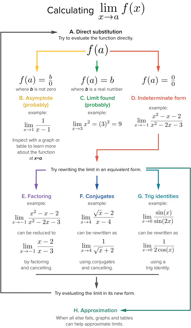
From these theorems, you can see that finding a finite limit is simply doing algebra manipulation of the function until you reach a point where you can substitute $x$ into your equation. The typical procedure to solve a finite limit can be found in .
Vertical asymptote
The tables in this section use $+$ simply to denote the fact that the number is $>0$ and similarly with the negative sign.
The limit of the multiplication between two functions, when it is at the asymptote, can be simplified in . Remember that multiplication is commutative and check if the limit exists in the first place or not. The table is pretty straightforward, as the signs are similar to multiplication between two numbers: two negatives get a positive.
| $\lim_{x\to a}f(x)$ | $\lim_{x\to a}g(x)$ | $\lim_{x\to a}[f(x) \cdot g(x)]$ |
|---|---|---|
| $+∞$ | $+$ | $+∞$ |
| $+∞$ | $-$ | $-∞$ |
| $-∞$ | $+$ | $-∞$ |
| $-∞$ | $-$ | $+∞$ |
The limit of a division between two functions $f(x)$ and $g(x)$ starts with two requirements: \[ \lim_{x\to a}f(x) \neq 0 \text{ and } \lim_{x\to a}g(x) = 0 \] After that, you need to check if the function $g(x)$ for $x$ approaches $a$ is larger than $0$ or not — you are checking the result that the whole function will dispense. The interaction between the limit of $f(x)$ and the sign of $g(x)$ can be found in . Note that you still need to pay close attention to which direction you are approaching $x$ and whether the limit exists at that point. Once again the signs are similar to typical division. ∞
| $\lim_{x\to a}f(x)$ | The sign of $g(x)$ | $\lim_{x\to a}\frac{f(x)}{g(x)}$ |
|---|---|---|
| + | + | +∞ |
| + | - | -∞ |
| - | + | -∞ |
| - | - | +∞ |
Trigonometric identities
As it is impossible to cover all of the identities, this section will list identities that are useful in AP Calculus exams. First, recall the definition of a few trigonometric functions:
Here are Pythagorean identities, which help when reviewing with a unit circle that displays trigonometric functions like :
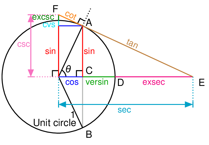
The $1^2=1$ was added to help the reader remember the connection to the original Pythagorean theorem $a^2+b^2=c^2$. You can work out more identities from the figure. Just in case you forgot, $\sin^2\theta=\sin(\theta)\cdot\sin(\theta)$ — it is the squared of the result of the function, NOT the $\theta$ inside the function.
The double-angle identities:
The half-angle identities frequently being mentioned but more often used for integral questions:
Finally, it is crucial to remember that the limit of most of the trigonometric functions as $\theta\to0$ is undefined. Can you see why?
Composite function limits
The standard theorem is:
If and only if the limit of $g(x)$ exists and $f(x)$ is continuous at $\lim_{x\to a} g(x)$: \[ \lim_{x\to a}g(x) = L \text{ and } \lim_{x\to L} f(x) \text { exists} \]
Remember: the theorem only stated about “moving” the limit inside and does not mention anything about the limit itself. Therefore, if you cannot apply the theorem, it does not mean that the limit does not exist so you should inspect the function instead.
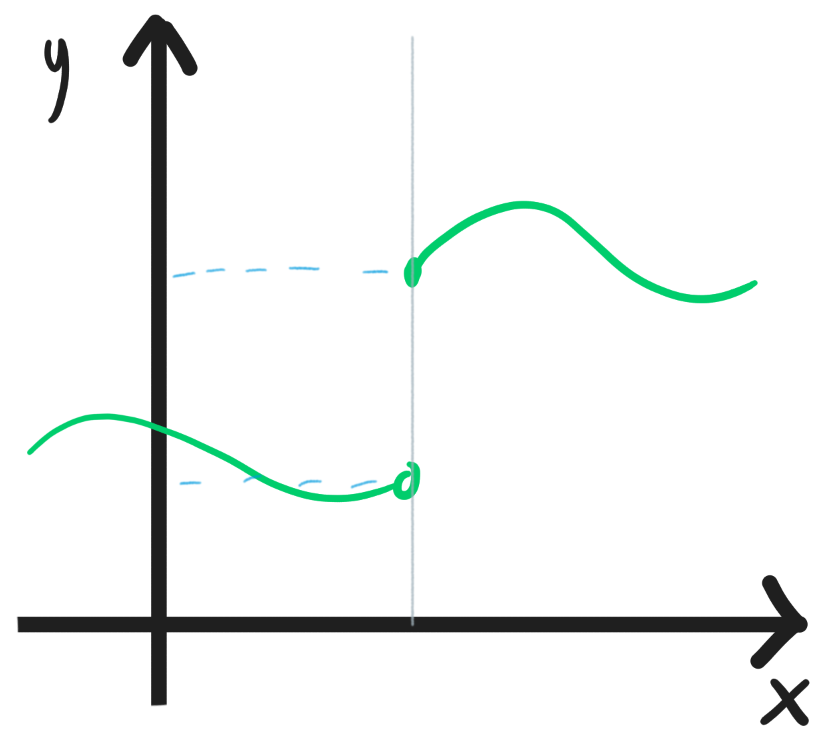
When inspecting the functions through graphs, it is best to put the two functions in two different graphs. Since the output of $g(x)$ is the input of $f(x)$, you can visualize it as if you “flip” the $g(x)$ y-axis to match with the x-axis of $f(x)$.
Finally, if the graph is discontinuous, it does not mean that the limit at that point does not exist. Slowly follow one-sided limits and see if they are equal.
Intermediate Value Theorem
If a function is continuous over an interval $[x_0, x_1]$, what you might be able to see is the fact that the function’s result (y-axis) will need to move from $y_1$ to $y_2$ — the function cannot “jump” because it is continuous. Therefore, this theorem guarantees that within $[x_0, x_1]$, you will find a value within $[y_0, y_1]$:
The f(x) may get out of the specified range (most notably quadratic equations), but we are certain that there exists at least one value satisfies our equation.
The squeeze theorem
Also known as the sandwich theorem, it helps calculate limits that are a bit weird. Suppose in an area that we know: \[ f(x) \leq h(x) \leq g(x) \] then for some real number $a$:
Read: If we certainly know that, inside the range we are evaluating, $h(x)$ is always between the other two functions, then if the limit of both $f(x)$ and $g(x)$ is equal to a number, then those two limits “sandwich” $h(x)$ to that same value.
For example, we have the following function with the graph from and : \[ x^2 \sin\left( \frac{1}{x} \right) \]
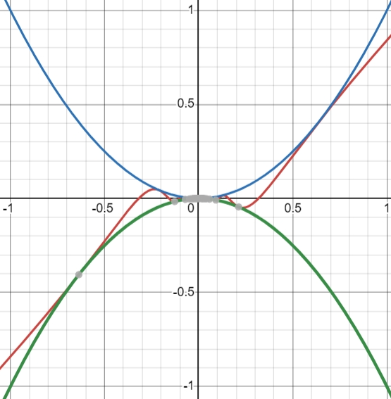
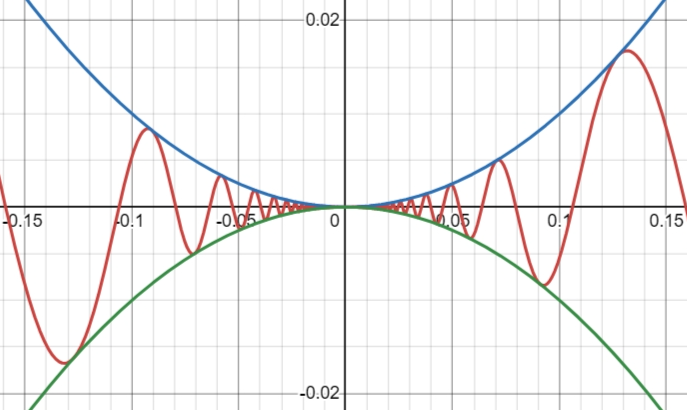
Of course, we can observe from the graph that the function approaches $0$ as $x\to0$, but what if we don’t have the graph? We know from the property of a sine graph that the coefficient at the front will determine the height of the graph. Therefore, we know that: \[ -1 \leq \sin(x) \leq 1 \Rightarrow -x^2 \leq x^2 \sin\left( \frac{1}{x} \right) \leq x^2 \] And we know that at $0$, $-x^2 = x^2 = 0$, therefore making: \[ \lim_{x\to0} x^2 \sin\left( \frac{1}{x} \right) = 0\]
Solving limits at infinity
There are two seemingly different ways to solve for infinite limits but behind the curtain, they are the same.
The intuitive way is to turn the function into a rational function (a function in the form $P(x)/Q(x)$). If the degree of the numerator is higher, then the limit is either positive infinity or negative infinity — you need to look at the sign of the $x$ with the highest degree since that $x$ will be the one that determines the direction of the equation. If the degree of the denominator is the largest, then the limit will head to $0$. If the degree of both are equal, divide the coefficients of the terms with the largest exponent: \[ lim_{x\to\infty}\frac{-5x^2+1}{3x^2-x} = \frac{-5}{3} \]
Finally, you can combine with the theorems mentioned above to adjust your answer properly. The reason this works is we are trying to find which term grows the fastest by comparing their degree; if they have the same degree, they “contested” each other to reach a ratio.
The algebraic way is to transform what you have into what you can evaluate. All the theorems from the solving finite limit section still hold unless specified otherwise.
\[\begin{aligned}
& lim_{x\to\infty}\frac{5x^2+1}{3x^2-x} \\
=&
lim_{x\to\infty}\frac{(5x^2+1) / x^2}{(3x^2-x) / x^2}
&\text{divide by } x^2 \\
=& lim_{x\to\infty}\frac{5+\frac{1}{x^2}}{3-\frac{x}{x^2}} \\
=&
\frac
{lim_{x\to\infty}(5+\frac{1}{x^2})}
{lim_{x\to\infty}(3-\frac{x}{x^2})}
&\text{apply the theorems} \\
=& \frac{5+0}{3-0} &\text{find the limit of each term} \\
=& \frac{5}{3}
\end{aligned}\]
It is once again crucial to remember that you cannot simply substitute $\infty$ into your equation and manipulate it as if it is a variable.
L'Hôpital's rule
If you think the derivative $f’(x)$ is simply a special transformation of the original function $f(x)$, we can use the derived function to solve a limit that is in the indeterminate form:
Here are the indeterminate forms that L’Hôpital rule can help with:
The conditions are, very obvious, the functions must be differentiable and the final limit must exist. Less obvious is the fact that you can only use this rule when $f(x)/g(x)$ is indeterminate.
You can take as many differentiations as it takes to solve the limit equation. You can also take the antiderivative but usually, that will result in a more complex function. Consider we have this example: \[ \lim_{x\to\infty} \frac{e^x}{x^2} = \frac{\infty}{\infty} \] Note that the derivative of $e^x$ is $e^x$, we can slowly transform our limit: \[ \lim_{x\to\infty} \frac{e^x}{x^2} = \lim_{x\to\infty} \frac{e^x}{2x} = \lim_{x\to\infty} \frac{e^x}{2} = \infty \] In the last step, we know that $e^x$ grows much more rapidly than $2$.
Derivatives
It is recommended that the reader understand about limits before proceeding.
Derivative concept
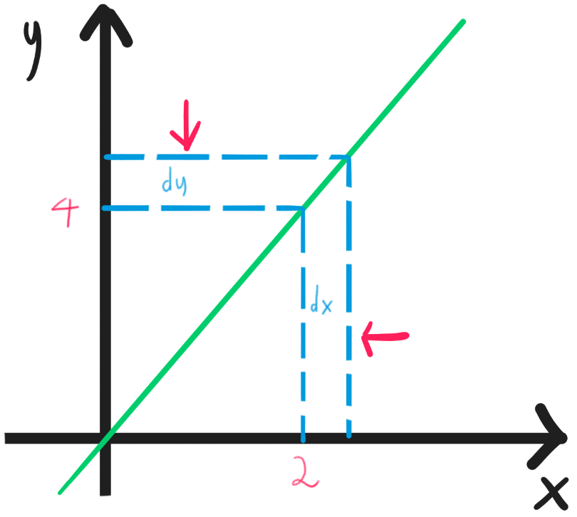
Today is a beautiful day to find the slope of a graph at a point. We remember that the slope between two points is the difference in the y-axis divided by the difference in the x-axis:
However, what we originally asked is the slope of a graph at one single point, therefore we need to move the two points as close as possible to each other (the definition of limit) until they are essentially one point similar to . Consider the fact that the y-axis essentially is the output of the function $f(x)$, making $\Delta y=f(x+\Delta x)-f(x)$, we can use limit to describe the fact that the difference $\Delta x$ is getting smaller and smaller ($\Delta x\to0$):
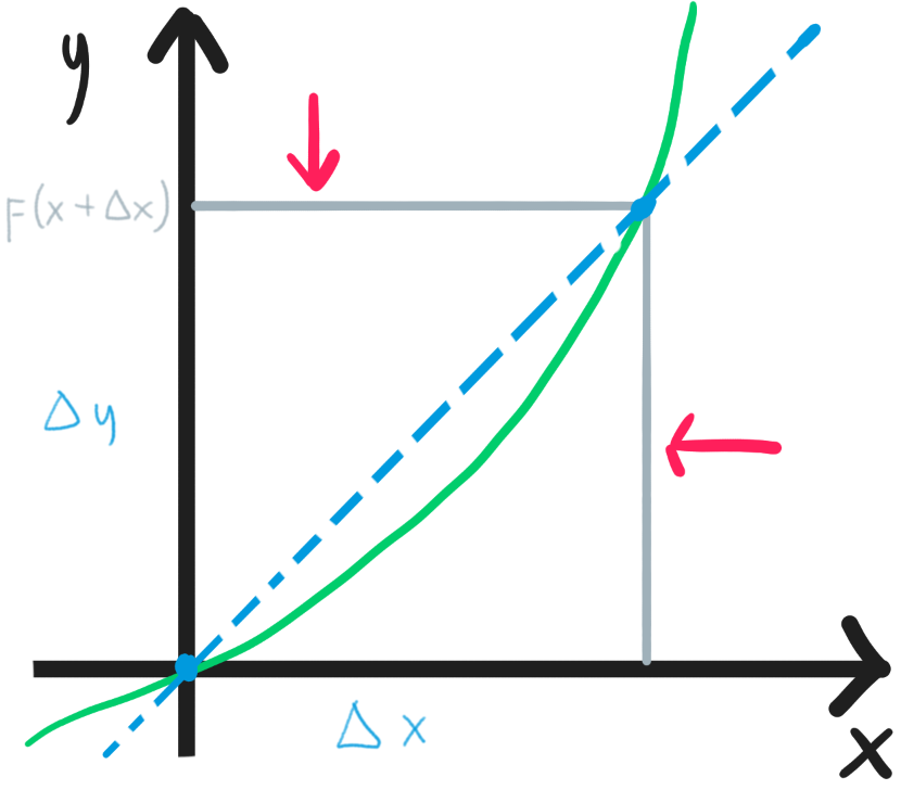
Other notations to highlight the fact that the derivative is simply the rate of change of a function at a point is:
This notation highlights the fact that the derivative is the ratio between the change in the y-axis and the change in the x-axis, giving you the ability to move $dx$ in a certain scenario. If you want to find the slope at a certain $x=c$, you can use the following notation:
Lastly, you can take derivatives as many times as you like. After all, if you take the derivative of a derivative, it simply showing the rate of change of the derivative function itself.
Derivative rules
In this section, instead of using the full notation $f(x)$, the function is simplified to $f$. The start of this section will simply provide a quick look-up sheet of the rules, while the latter part will explain the intuition of some harder rules.
A note: before you do any derivative manipulation, consider simplifying the function. For example, we have: \[ [(x+1)^2]’ = [x^2 + 2x + 1]’ = 2x + 2 \] If you were to manipulate the original equation as a composite function the derivative would be much messier.
Multiplication by a constant:
The sum and difference rule are a bit anti-climatic:
The product rule can be remembered by the phrase “Left-D right, right-D left”:
The quotient rule was found by expanding the derivative’s limit definition. The numerator is almost similar to the product rule, except with a minus; if you imagine we are multiplying $\frac{f}{1}\frac{1}{g}$, then the $g^2$ is almost like trying to use the reciprocal to cancel out the denominator. I know this explanation is not accurate, but it is a good way to visualize the rule during tests.
The reciprocal rule is another rule that is a bit hard to digest, but luckily rarely seen:
It is also appropriate to recall the fractional exponent rule and negative exponent rule:
Which will be useful when utilizing the power rule:
You can remember that the power rule “flattened” our exponent graph by one degree.
The chain rule in a wordy notation but the one that gets across my mind is: assume we have $u=g(x)$ and $y=f(u)=f(g(x))$ then the derivative is:
This means that “the derivative of $f$ plug in original $g$ times the derivative of $g$ plug in $x$”. You can feel it showcases a “staircase” approach to the composite function.
The L’Hôpital rule is used when finding the limit at a point with an indeterminate result (read more about its usage in ):
This means the limit of a quotient of two functions equals the limit of the quotient of the derivative of those two functions.
When all rules fail, you can always use the original derivative definition in equation
Visualizing the product rule
Assume we have two functions: $g(x)$ and $h(x)$, and $f(x)=h\cdot g$. Because it is the multiplication between two functions, you can think of $f(x)$ as the area of a rectangle with $h(x)$ and $g(x)$ as two sides, similar to .
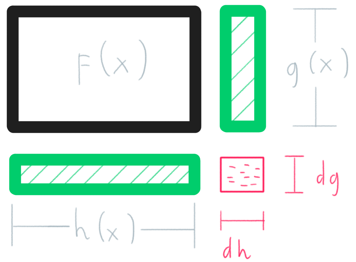
To calculate the rate of change at that point, we need another point $dx$ away from $x$ and $dx\to0$. Furthermore, we need to consider how our two functions “react” to $dx$. We deduct from the formula of derivative: \[ \frac{dh}{dx} = h’ \Leftrightarrow dh = h’ \;dx \] A similar transformation can be made with $g(x)$. What $dh$ is showing here is how much the result of the function $h(x)$ would increase for a change in $x$ — $dh$ is the change we have when we move $x$.
Label the additional area $df$: \[ df = g \cdot dh + h \cdot dg + dh \cdot dg \] We can expand the entire equation to: \[ df = g(h’ \;dx) + h(g’ \;dx) + (h’ \;dx) \cdot (g’ \;dx) \] We want to find the ratio at that point $df/dx$, so we divide both sides by $dx$: \[ \frac{df}{dx} = g \cdot h’ + g’ \cdot h + h’ \cdot g’ \;dx \] Because $dx\to0$, we can eliminate that term: \[ \frac{df}{dx} = gh’ + g’h \Rightarrow \frac{d}{dx}(gh) = gh’ + g’h \]
Visualizing the chain rule
An anonymous professor once said: “Using the chain rule is like peeling an onion: you have to deal with each layer at a time, and if it is too big you will start crying.”
Assume we have $g(h(x))$. We can imagine these two functions like a production line: we put in the raw number $x$, and then the function $h$ will “process” the input before passing it to $g$, after which the output will then be given. This production chain can be visualized in . Note that now we denote a tiny change in our input as $dx$, a tiny change in our output as $dy$, and our ultimate goal is to find the ratio $dy/dx$.
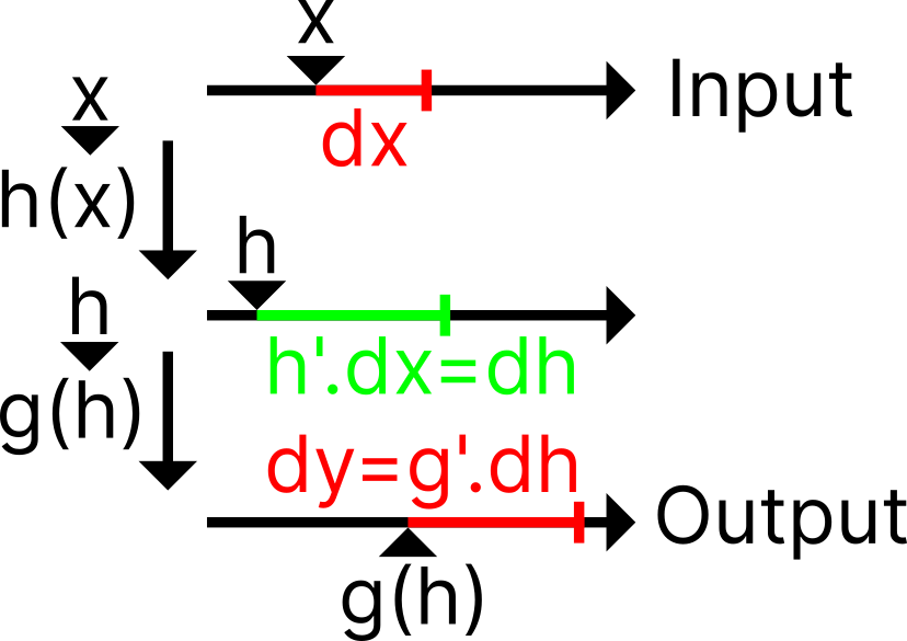
As we increase our input by a $dx$ amount, it will increase the output of the function $h$ by a $dh$ amount. Similar to the product rule, we manipulate our derivative ratio $dh/dx$ to calculate that change in the output: \[ dh = h’(x) \;dx \] Repeat that same process with the function $g$, but now you have to remember that the input is no longer $x$, but $h$ and a tiny change $dh$: \[ dy = g’(h) \cdot dh \] Expand $dh$, we have: \[ dy = g’(h) \cdot (h’ \;dx) \] Finally, because we ultimately want to find the ratio of the changes, we divide both sides by $dx$ and expand the fact that $h$ is simply $h(x)$: \[ \frac{dy}{dx} = g’(h(x)) \cdot h’(x) \] If you think of $dg/dh$ as “derivative of $g$ when plugging in $h$”, another interesting way to write this: \[ \frac{dy}{dx} = \frac{dg}{dh}\frac{dh}{dx} \]
Derivative of common functions
A constant will have a slope equal to $0$:
A line will have a slope similar to its… slope. This is similar to $m$ in the form $y=mx+b$:
The derivative of a square root:
Exponential functions with $x$ as the exponent. Further explanation can be found in Euler’s constant and the natural $\log$:
Logarithms:
Trigonometric functions:
Additional material
It is recommended that you explore for the inverse concept of derivative: anti-derivative. For other additional reading material connecting to calculus as a whole, place look at .
Integrals
It is an absolute requirement that the reader understands derivatives, which in turn requires the knowledge of limits.
Why antiderivative is integral?
This section is not necessary to understand the concept of integral, so the reader feels free to skip it. However, this section will provide an in-depth examination of how mathematicians came up with the connection between antiderivative and integral — we are going to construct calculus from the ground up. If that is the question you have in mind, please continue to read this section as the author has rewritten it thrice now.
Assume we have a graph $f(x)$ and an unknown function $A(x)$ that represents the area under $f(x)$ between the y-axis and the input. We will split into two situations and each situation will explain a different component of integration to construct the full image:
The main function is zero-degree (constant)
If we have $f(x)=c$, the graph of our constructed function will look like . If we were to find the area between $0$ and $a$, we could simply calculate $A(a)$ to get the result.

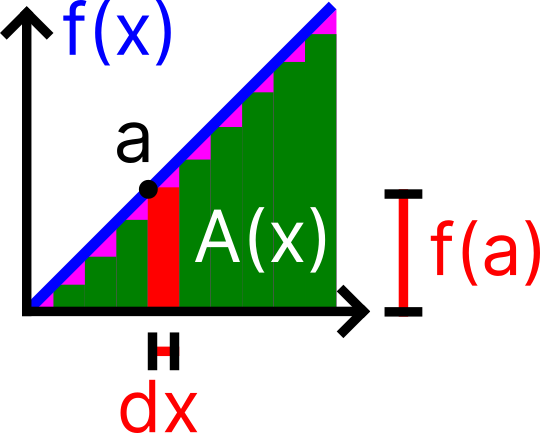
If we move $a$ a $dx$ amount to the right and want to find the area at that point, we plug $A(a+dx)$. If you look at the red rectangle on the figure, there are two ways to interpret that area:
- It is the area of $A(a+dx)$ subtracted by $A(a)$
- It is the area created by the increase in the variable $a$ (which is $dx$) multiplied by the height of that area $f(a)$ (in this case, we plug the number in to find the height).
And clearly, those two are mentioning the same area, so we can state that they are equal: \[ A(a+dx)-A(a) = f(a) \;dx \] We can generalize the point we selected by replacing $a$ with $x$: \[ A(x+dx)-A(x) = f(x) \;dx \] Then re-arrange the equation: \[ \frac{A(x+dx)-A(x)}{dx} = f(x) \] Hang on… that essentially stated that the slope of $A(x)$ is the value of $f(x)$; on the other hand, it stated that essentially $f(x)$ is the derivative of $A(x)$! Despite $A(x)$ being unknown in the beginning, we can find a function whose derivative is $f(x)$ to get $A(x)$. Thus, the antiderivative is the area under the graph.
The main function is first-degree (linear)
Alright, we have seen the connection between $A(x)$ and $f(x)$, but where are the $\int$ sign and the final $dx$? Assume $f(x)$ is a linear equation with a graph similar to . Notice that now our area function will need to account for both the green rectangle and the pink triangle at the top of every rectangle.
If we want to find the area under $f(x)$ from $0$ to $a$, we will need to add the area of all of the slices between $0$ and $a$. The area of each green rectangle is $f(x) \;dx$ and we want to find the sum of all of those areas from $0$ to $a$:
\[
\int^a_0 f(x) \;dx + \text{pink area}
= A(a)
\]
As you can see, the $\int$ acts both as a $\Sigma$ notation for the sum of the rectangles and $\lim_{dx\to0} f(x)\;dx$
Note that the smaller the $dx$, the finer we slice our area, making our pink area approach $0$ and our summation of the green area closer to the actual area. Algebraically, this is because $f(x)=dA/dx$ so the left term will cancel out $dx$, while the pink area will still be multiplied by $dx$ (the base width of the triangle). Eventually, we have: \[ \int^a_0 f(x) \;dx = A(a) \]
If we have another point $b>a$, and we want to find the area from point $a$ to $b$, we simply find the area of point $b$ and minus it by the area at $a$: \[ \int^b_a f(x) \;dx = A(b) - A(a) \]
Integration concept
Starting with a geometry intuition: think of a paper. If you look at a paper from the edge, it has a very tiny thickness. However, as you stack the papers together, eventually those tiny thicknesses will create an area on the side: you can measure the height of the stack and multiply it by the edge’s length to get the stack’s edge area.
Integral is the antiderivative of a function, which helps us find the area under a curve by chopping it into thin sheets and stir-frying it… wait sorry wrong note… Ehem…
Integral helps us find the area under a function $f(x)$ by slicing it into many small pieces with equal $dx$ thickness and height of $dx$. As $dx\to0$, our approximation of the area will get better and better; at some point with extremely small $dx$, the value would just be the sum of all small segments of $f(x)$. Similar to our paper example from above: as we continue to stack the papers, the sides will eventually create an area. To tell that $F(x)$ is the indefinite integral of $f(x)$, we use
The reason we have $C$ is because any constant will have its derivative as $0$, so both $F(x)+1$ or $F(x)+3$ will have the the derivative as $f(x)$. To express that we have a lot of possible antiderivatives, we use the constant $C$. When solving integrals, most of the time you can simply add the integration constant at the very end when answering the question instead of accounting it for every small step.
The notation we used above is indefinite integral which expresses a function without any particular input and does not spit out any number. If we want to find the area of a particular region $[a,b]$, we will use a definite integral to denote $a$ as the lower bound and $b$ as the upper bound. Since we have $F(x)$ as the area function from $0$ to $x$, we find the area of $[0,b]$ and then subtract it by $[0,a]$ to get the interested area:
Note that the $C$ was conveniently cancelled, so we can ignore that.
Another important thing to remember is integral is the signed area under a function. What that meant is that if the function $f(x)$ ever dipped below $0$, then the area between the x-axis and $f(x)$ will be considered negative. If you want the area in general without that subtraction, consider splitting your integral into two: calculate the positive area then add it to the absolute value of the negative area.
Notation-wise, because integration is the sum of $f(x)\;dx$, it is also appropriate to remember that the $dx$ is still a part of the integral
A final word of this section: antiderivative (indefinite integral) is simply the function $F(x)$ without any real value, while definite integral is the result of plugging in values into our indefinite integral. Those two terms are usually used interchangeably, but they are slightly different.
Integration rules
Note that the lowercase $c$ in this section is different from the integral constant $C$ (uppercase). Generally, the integral of a function will have a higher degree and will be a bit more complex but in academic settings, the teachers will usually make integration easy.
The sum rule and the similar difference rule are almost universal at this point after you learn limit, derivative, and integral:
Is it quite fascinating to see that the integral sign and the $dx$ are similar to being distributed across the terms?
Multiplication by a constant:
The power rule has a requirement that $n \neq -1$:
Integration by parts is useful when you can separate your functions into two parts and multiply those together. Assume you found two functions $u(x)$ and $v(x)$:
You can specifically define two functions as $u$ and $v’$, and solve for $u’$ and $v$ individually:
When writing the result, remember: alternate both $u$ and $u’$, but you only use the solved $v$.
Integration by substitution or the reverse chain rule requires you to set up your chained function in a particular way. Assume: \[ g(x)=u \qquad g’(x) \;dx=du \] We can use $u$ as an input placeholder and compute our integral as:
After that, solve the integral normally (remember the variable is now a placeholder $u$) before substituting $g(x)$ back into the equation.
The power rule
The intuition has $nx^{n-1} = (x^n)’$ as the derivative’s power rule. However, the left side is $n$ times larger than our function inside the integral. If we were to divide both sides by $n$, then the input would be the original function stated in the rule. Of course, the $n$ is offset by $1$ because we put it relative to the derivative on the right side. \[ nx^{n-1} = (x^n)’ \Leftrightarrow x^{n-1} = \frac{(x^n)’}{n} \Rightarrow^{\text{-ish}} x^{n} = \frac{x^{n+1}}{n+1} \] Such a way of thinking will work, but as you can see, it is not accurate when you need to insert that “-ish” into the equation. As for the reason it is not accurate, did you realize that the final equation somehow dropped the derivative bracket?
Integration by parts
While it is true that we need to have $C$ for every integral result, it is not necessary in the case of the inner integrals $\int v\;dx$ because the $C$ will eventually cancel out.
It is important to identify which $u$ and $v$ to use to make the derivatives and integrals easier — you should choose a $u$ that gets simpler when you differentiate it and is similar to $v$ integration. A rule to remember is I LATE. You should choose $u$ based on which of these comes first:
- I: inverse trigonometric functions such as $sin^{-1}$
- L: logarithmic functions like $\ln(x)$ or $log(x)$
- A: algebraic functions like $x^2$ or $x+1$
- T: trigonometric functions such as $\sin(x)$
- E: exponential functions such as $e^x$ or $3^x$ ($x$ as the power… you don’t want to give something unknown the power)
The formula originates from algebra manipulation of the original product rule:
\[\begin{aligned}
&(fg)’ = fg’+f’g \\
\Leftrightarrow& fg’ = (fg)’-f’g \\
\Leftrightarrow&\int fg’\;dx = \int(fg)’\;dx-\int f’g\;dx
&\text{Take the integral of every terms}\\
\Leftrightarrow&\int fg’\;dx = fg -\int f’g\;dx
&\text{Derivative cancels the integral}\\
\end{aligned}\]
Integration by parts trick: the tabular method
This is a quick trick to calculate the integral function that was set up according to our stated format $\int uv\;dx$ of the integration by parts rule. It is recommended that the reader find an online resource with videos to explain as it is much easier to understand with an interactive format. A recommended video was included in the additional material section.
It is best to show the procedure as an example. Let’s say we have the following integral: \[ \int x^3\sin x \;dx \] We identify $u=x^3$ and $v=\sin x$. Next, we set up the . For every row on the $u$ column, we take a derivative of the previous row; similarly, we take the antiderivative for every $v$ row. For the sign, you can either denote it on the arrow, make a separate column for it, or negate the results in the $u$ column; the last row of the sign column was left empty as a reminder that you will not take the last derivative into the final result.
| Sign | $ u $ | $ v $ |
|---|---|---|
| + | $ x^3 $ | $ \sin x $ |
| - | $ 3x^2 $ | $ -\cos x $ |
| + | $ 6x $ | $ -\sin x $ |
| - | $ 6 $ | $ \cos x $ |
| $ 0 $ | $ \sin x $ |
Take a look at and now look at what one should get as a result. It is easier to remember the method visually than a wordy description.
\[\begin{aligned}
\int x^3\sin x \;dx =
&+ x^3 (-\cos x) \\
&- 3x^2 (-\sin x) \\
&+ 6x (\cos x) \\
&- 6 (\sin x) \\
=& -x^3\cos x + 3x^2\sin x + 6x\cos x - 6\sin x
\end{aligned}\]
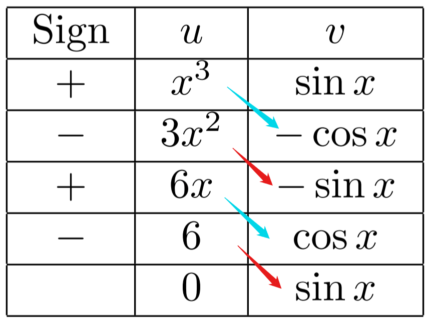
You need the $u$ column to eventually reach $0$ to make this method work. In case your table gets too long, maybe consider using the original integration by parts formula (). Furthermore, do not worry about accidentally going past the stop point, as the $0$ in the $u$ column should remind you that $a\times0=0$.
Integration by substitution
The listed formula somehow subtlety cancelled out everything but in reality, it is just simply an expansion of the derivative $du$ itself. Let’s start fresh from an integral:
\[
\int \cos(x^2) \cdot 2x \;dx
\]
We can define $u$:
\[
u = x^2
\]
Therefore $u’$ or the derivative of $u$, notated with small changes in $du$ is:
\[
\frac{du}{dx} = 2x
\Leftrightarrow
dx=\frac{du}{2x}
\]
Replace $dx$ into our integral, we can see the $2x$ were cancelled out nicely, making all the variables inside the integral become $u$ instead of $x$. After that, we can calculate the integral with our input variable as $u$, then substitute $u$ back to answer:
\[\begin{aligned}
\int \cos(x^2) \cdot 2x \;dx
&= \int \cos(u) \cdot 2x \;\frac{du}{2x} \\
&= \int \cos(u) \;du \\
&= \sin(u) + C \\
&= \sin(x^2) + C
\end{aligned}\]
Note that most of the time, it is not possible to start with an already set-up function but it is okay: you can just go ahead and select a convenient $u$ and replace $dx=du/u’$. We have this example:
\[\begin{aligned}
\int x\sqrt{x-1} \;dx
&= \int x\sqrt{u} \;du
\qquad\text{Define } u=x-1 \text{ and } du=dx \\
&= \int (u+1)\sqrt{u} \;du
\qquad\text{From the original definition: } x=u+1 \\
&= \int (u+1)u^{\frac{1}{2}} \;du \\
&= \int u^{\frac{3}{2}} + u^{\frac{1}{2}} \;du \\
&= \frac{2}{5}u^{\frac{5}{2}} + \frac{2}{3}u^{\frac{3}{2}} \\
&= \frac{2}{5}(x-1)^{\frac{5}{2}} + \frac{2}{3}(x-1)^{\frac{3}{2}}
\qquad\text{Substitute } u=x-1 \\
&= \frac{2}{5}\sqrt{(x-1)^5} + \frac{2}{3}\sqrt{(x-1)^3}
\qquad\text{Add integration constant}
\end{aligned}\]
Integral of common functions
The constant function has a similar representation to the where the integral will increase the degree of a function. It is the power rule in .
If you continue to expand the power rule, we will have an integral for linear function and a squared:
The reciprocal function can be used for general situations or when $n=-1$ for the power rule:
Exponential with Euler’s number is quite easy to remember if you remember that its derivative is always itself (with the $C$):
If we have the variable as the power, natural log once again came up:
And if we put a natural log on the table after appearing in so many equations, we have its integral as:
Trigonometric functions can be remembered by recalling the original derivative trigonometric functions:
Additional material
- A YouTube playlist by 3Blue1Brown to help with the visualization of constructing derivatives (as well as other calculus concepts): Essence of calculus
- An in-depth look into the proof and connection between derivatives and integrals: https://en.wikipedia.org/wiki/Fundamental_theorem_of_calculus
- The tabular method explanation video: https://www.youtube.com/watch?v=Yyic5aaXGaw
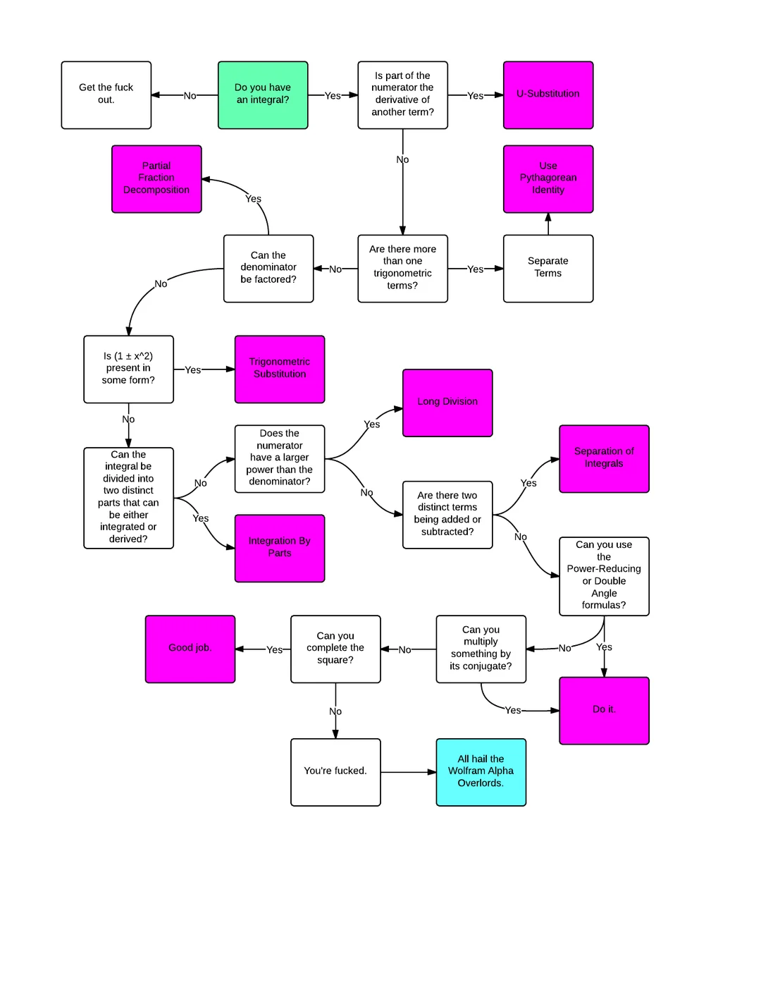
- A strongly worded flowchart to solve integrals can be found in
Chemistry
Useful Figures and Formulas in Chemistry
The periodic table of the elements is arguably one, if not, the most important thing to have when learning chemistry. For the high school level, the most useful periodic table is the one that has ion charges of the elements.
A table of common symbols used in formulas can be found in
| Symbol | Name | Unit | Explanation |
|---|---|---|---|
| n | Number of moles | mol | See section |
| m | Mass | g | |
| M | Molarity | g/mol | See section |
| V | Volume | L | |
| %A | Percentage composition of element A | % | See section |
| D | Density | g/l |
Formulas
In this section, each name will followed by a reference to the equation (or the section) that explains the formula. There are no units included for the sake of memorization but you should always keep the unit in the back of your head, or better yet, remember the conversion factor procedure.
Number of moles when given mass and molar mass ():
Number of moles of a gas in standard condition ():
Stoichiometry
Stoichiometry simply means that we are dealing with chemical reactions and the quantitative data from such reactions (like weight, volume, number of atoms, etc…).
The mole — the central number of chemistry
How many items are there in a triplet? $3$. How much is a dozen? $12$. Now we have a new definition:
Similar to how half a dozen is $0.5\times12=6$, you can tell other scientists that you have a certain number of moles of something. Note that a mole is still a quantity and not a unit — you have a mole of something. As a conversion factor, a mole is:
A mole of atoms of an element acts as the central unit to convert between different units or elements in a reaction.
Molar mass is the mass of $1$ mole of an element while the formula mass of a compound is the sum of all atoms in that compound. They are both similar in value but different in the unit: molar mass’s unit is usually in grams per mole while formula mass is in the atomic unit, which is $1/12$ the weight of a carbon atom (or about $1$ hydrogen atom). The atomic unit will be abbreviated as “u” throughout this note.
To calculate the number of moles, you can see how many times the molar mass you have of the element A:
$1$ mole of any gas at standard temperature and pressure or STP occupies exactly $22.4$ litres. That property only appears for gasses but not liquids or solids. If you want to calculate the number of moles in a volume of gas:
Molarity is the number of moles of the chemical per litre of a solution. It indicates how many moles of the chemical are presented in a litre of a solution — similar to density but in this case, it is the number of atoms over 1 litre of the solutions. Because a solution will include both the chemical and the water, the actual amount of water present in the solution is not $1$ litre — you add water up to $1$L, NOT $1$L of water.
The relationship between a mole and the chemical formula is in the proportion. For example, the element dihydrogen monoxide
Composition analysis
Before calculating anything, it is usually appropriate to know the chemicals you are using. The first thing to realize is that not all atoms are similar in weight; consider a composition of H₂ and O, the O will make up most of the mass in a molecule — this happened because one O elements weight $16$u while a hydrogen atom weights at about $1$u.
An example to determine the percentage composition or how much each element takes up the total mass in a water molecule: first calculate how much each element weights in the entire compound: \[ 1\text{g H/mol H}\times2=2\text{g H/mol H}_2\text{O} \qquad 16\text{g O/mol O}\times1=16\text{g O/mol H}_2\text{O} \] In this stage, we calculate the weight of individual items that make up our compound. From the formula to create $1$ mole of water, you will need two moles of hydrogen and $1$ mole of oxygen — this is proportional to having 2 atoms of hydrogen and 1 atom of oxygen. Honestly, you could just make this calculation using atomic units instead of grams and it would work about fine but for the sake of accuracy, please refrain from doing so. Anyway. we will now total up the weight of individual elements to get the weight of the entire compound before calculating the percentage: \[ 2 + 16 = 18\text{g H}_2\text{O/mol H}_2\text{O} \] \[ \%\text{H} = \frac{2 \text{g H}}{18 \text{g H}_2\text{O}}\times100 = 11\%\text{H} \] Despite you need two atoms of hydrogen to build a single molecule, clearly that single hydrogen atom takes up more weight.
The general formula to calculate the percentage composition with the mass of an element $m_A$ and the compound’s mass $m_{AB}=m_A+m_B$ is:
To calculate an empirical formula, we start by pretending we have $100$g of the substance: $11$g of that substance would be hydrogen and $89$g would be oxygen. We now divide each of those numbers by the molar mass to obtain the number of moles in that mass: \[ 11\cancel{\text{g H}} \frac{1\text{mol H}}{1\cancel{\text{g H}}} = 11\text{mol H} \qquad 89\cancel{\text{g O}} \frac{1\text{mol O}}{16\cancel{\text{g O}}} = 5.5625\text{mol O} \] Then divide them by the smallest factor (in this case $5.5625$) to get the ratio between elements: \[ 11/5.5625=1.977 \] Because of the estimations in our equation, it is appropriate to assume that it is 2 moles of hydrogen for every oxygen atom or H₂0.
If you were to simplify the process of calculating empirical formula into an equation, define the formula AxBy and $n_A$ is the molar mass of A, we have the ratio:
Chemical equations
A chemical equation usually indicates the proportion of the chemicals that participate in a reaction, essentially showing the mole of particles you need.
Electron Configuration
Introduction: The modern model of atoms
This section is for a simplified explanation of what is going on. It is not required if you are in a hurry but is highly recommended to grasp the deeper understanding of the explanations in the latter sections.
Most of us are used to the fact that an electron flies around the nucleus in a fixed orbit. This is unfortunately an oversimplification of what happened but for a good reason. Throughout this chapter’s model, an electron can move freely around a region rather than flying in a predetermined orbit. Every time you “observe” an electron, you take a picture of it which shows its position in space. As you take more pictures, you will eventually see where it is most likely to appear, and that is how you establish the orbit
The first four atomic orbital shapes that you will see are s, p, d, and f. For larger atoms, there will be more electrons which require more space to be in, which will create more diverse region’s shape (likewise, the outer shell in the classic atom model has more electrons than the inner shell). Each atomic orbital can store up to 2 electrons and will be filled from the smallest orbital to the biggest orbital (which will be called a “shell”). Lastly, the electrons are shy and they would love to occupy an orbital to themselves if possible using Hund’s rule.
Of course, what is being said is still a simplification but it is enough for you to grasp the idea of what we are doing in this chapter. Particularly, the given model does not address the wave-particle duality of quantum mechanics nor the complexity of electron orbit; for your information, all of that is stepping on the line between physics and chemistry. Now, this section is the general analogy for you to understand but the latter sections will have a more academic approach to the topic for you to take tests.
Quantum numbers
There are three unique quantum numbers to describe an atomic orbital; this can be extended to describe an electron using the orbital it is in and its spin (the fourth quantum number). The Pauli exclusion principle says that each orbital only has 2 electrons with a different spin, which means that the four quantum numbers are essentially the ID of an electron.
The principal quantum number ($n$) indicates the relative size of the atomic orbital. This is relative to the “shell” of the electron in the classic atom model, so as the number of shells increases, there will be more electrons which leads to more atomic orbital. Most of the time, a higher $n$ means that the orbital has higher energy and the electron will spend more time farther from the nucleus.
The azimuthal quantum number ($l$)
As far as this chapter is concerned, you will mostly refer to this number using letters instead. Starting from $l=0$ and going up, we will refer to the subshell as s, p, d, f, g, h, and i; the letters after the g sub-shell follow in alphabetical order—excepting letter j and those already used. At the introductory level, the subshell f will likely be the highest $l$ you will ever see.
The magnetic quantum number ($m_i$) tells us the orientation in space of a given atomic orbital. This number is fortunately unimportant for our electron configuration topic, but keep in mind that an orbital shape can have multiple different orientations, usually based on the three 3D axes: $x$, $y$, and $z$.
As you can see from the formula, the number of possible $m_l$ (hence the number of electrons) grows pretty quickly.
Those there quantum numbers are enough to indicate which orbit you are talking about. It is suitable to remember that there are many possible orientations of an atomic orbital and many orbits with relatively the same size; similarly, in classical words, there are many orbitals in a subshell and many subshells in a shell. At this introductory level, many terminologies from the classical model are often used interchangeably with the vocabularies from the quantum mechanics model, so do not worry about using the correct word… yet.
The spin quantum number ($m_s$) as the fourth quantum number indicates the quantum spin of a particle or in this case, an electron. Because an atomic orbit can have two electrons with a different spin, this number is necessary to indicate which electron you are referring to.
Orbital diagram
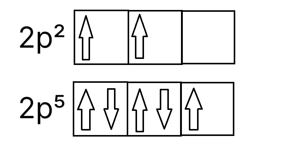
An orbital diagram is used to represent how many electrons are there, and what orbit they are in. Each box here represents an orbit, which can store two electrons drawn by two arrows; if there is only one electron, that electron will have up spin. represents how electrons slowly fill from the smallest to the biggest orbit (from 1s to 2s). It is once again important to remember the Pauil’s exclusion principle and the fact that the two electrons that share the same orbit should have a different spin.
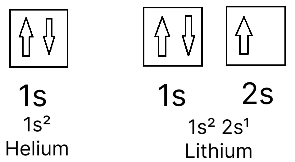
We group orbitals from the same subshell by connecting the sides of the orbital boxes. The Hund’s rule dictates how we should fill the atomic orbitals from the same subshell:
Every orbital in a sublevel is singly occupied before any orbital is doubly occupied.
In simple terms demonstrated by , you should fill all the orbitals in the same subshell with electrons of the same spin (in most cases, up spin) before putting in the opposite spin.
The number of orbitals per subshell is based on the third quantum number mentioned above: it is the number of possible values for $m_i$. The general formula for the number of atomic orbitals based on the second quantum number $l$ is:
Multiply the result by 2 and you get the number of electrons a subshell can hold.
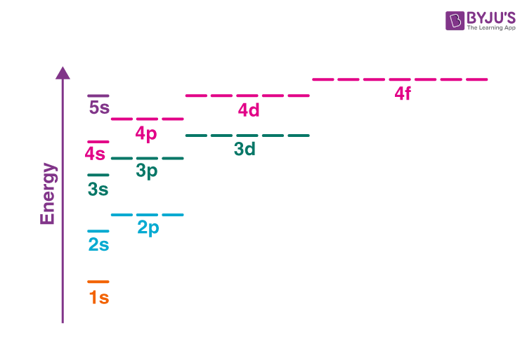
Another thing you need to keep in mind is the Aufbau principle (“Aufbau” in Germany translates to “build up”, which suits its purpose of building electron configuration from the ground state up):
When filling orbitals, the lowest energy orbitals available are always filled first.
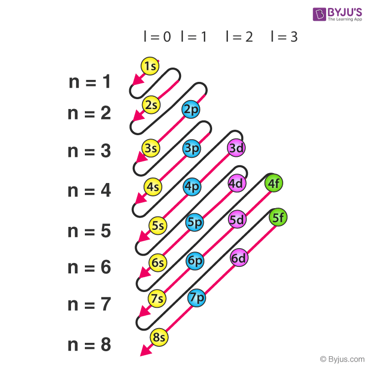
This principle is here to warn you of the fact that the subshell’s energy level is not in order. Yes, the order inside a shell follows the basic order based on $l$; however, an example would be the subshell 4s has a lower energy level compared to the 3d subshell. This is a reminder that $n$ is simply to show you the relative size of the orbit (compared to a similarly shaped orbit) while $l$ is the shape — this is why the terminology “shell” is confusing in this case, as we tend to think they are orderly stacked but in fact, they are not (). Luckily, there is a trick to remember the energy level, presented in ; the Aufbau principle starts to kick as we reach scandium, the first transition metal in the periodic table.
And just like any principle in chemistry, there are exceptions to the Aufbau principle. These exceptions are not very related to chemistry but it should not come as a surprise when encountering them.
To summarize this section, here is the list of things to think about when drawing an orbital diagram:
- Count how many electrons you need, then divide by 2 to have the number of boxes you will need to have
- Draw out the boxes with the correct shell subshell configuration. A simple tip to remember is 1, 3, 5, 7 for the s, p, d, and f subshell
- Fill the subshell: fill the entire subshell with up-spin electrons before filling it with down-spin (or vice versa for special cases)
- Stop when you already put down enough electrons, check if your element has a special case (usually question-dependent special cases)
Electron configuration
Taking from , lithium’s electron configuration has 3 electrons on two separate subshells — we write the number of electrons per subshell as a superscript after the subshell’s notation. If we have $x$ as the number of electrons in a subshell, the general format for a subshell’s electron configuration is:
This makes the electron configuration for Li which has 3 electrons as: \begin{equation} 1s^2\;2s^1 \end{equation}
Regarding the Aufbau principle, there are conflicting sources regarding whether you should sort according to the energy level or the shell’s number order. This is up to you but consult your instructor for their preference. However, sorting by shell order is especially useful for writing the electron configuration of ions (which will be discussed later).
The core notation allows us to condense the electron configuration of elements based on the last noble gas before the element in the periodic table. This is because of the property where noble gas has a full valence shell. For example, sodium follows immediately after neon, so we can simplify to the core notation with warping Ne in a square bracket: \begin{equation} 1s^2 \; 2s^2 \; 2p^6 \; 3s^1 \rightarrow [\text{Ne}] \; 3s^1 \end{equation}
The valence shell (the outermost shell) is also how chemists name the blocks from the periodic table. From the example above, Na is clearly from the s block, as its outermost subshell is s. Once again, keep in mind the Aufbau principle and the outermost shell is not necessarily the shell with the highest $n$ quantum number.
Recall that a cation has fewer electrons (positively charged) and an anion has more, which will in turn remove some electrons from the electron configuration. For only cations, sort the neutral atom’s electron configuration from the smallest to the largest, disregarding the Aufbau principle. After that, simply add or remove the electron according to your sorted order. Because of that, Sn4+ should not be written as [Kr] 5s2 4d8 but instead as: \begin{equation} \text{[Kr]} \; 4d^{10} \end{equation}
If an ion has the same electron configuration as another neutrally charged element, we call it isoelectronic with that element.
Physics
Mechanical Force, Work, Power, and Energy
This is a chapter to distinguish the four concepts and draw a connection between them. This chapter concerns mechanical physics so you might need to look somewhere else for thermal and electrical energy.
Force
Force can be described as a push or pull on an object, usually denoted with $\vec{F}$. Force is a vector, so it has a direction and a magnitude.
Net force is the sum of all forces being exerted on one single object. If you don’t see an object being moved (like when you are pushed against a heavy object), it is because your $\vec{F}_{net}=0$, since all forces cancel out each other.
Thanks to Sir Issac Newton, we have three Newton laws of motion that describe the way forces are described in physics:
Newton's first law
An object at rest remains at rest, or if in motion, remains in motion at a constant velocity unless acted on by a net external force
In short, if the $\vec{F}{net} = 0$ then the object will continue to do what it is doing. This law resulted in the existence of momentum: you don’t need to do anything to keep an object moving in a no-friction environment — it is the _change in motion that requires a force to alter the object’s movement.
Newton's second law
The algebraic version of Newton’s second law is:
With $m$ being the mass and $\vec{a}$ being the acceleration vector.
A real-life intuition for this is you need to push a heavy car a lot stronger for it to move (accelerate) compared to pushing a shopping cart.
Newton's third law
If body $A$ exerts a force $\vec{F}$ on body $B$, then $B$ simultaneously exerts a force $-\vec{F}$ on $A$:
A common misconception is that the action and the reaction forces cancel each other out. This was cleared out by the law’s equation because the forces were considered on two different systems. For example, when pulling down on a vertical rope, a climber is exerting a force on the rope ($\vec{F}{AB}$), while the rope is pulling upward _on the person ($-\vec{F}{BA}$). When you draw a free-body diagram, the downward vector is the gravitational vector pulling _on the person, so it is not $\vec{F}{AB}$. Repeat: $\vec{F}{AB}$ DOES NOT CANCEL $-\vec{F}_{BA}$.
Bra–ket Notation
Introduction
The bra–ket notation provides a separation from the term “vector” that is used for quantities like displacement or velocity — these vectors tend to be related to the three dimensions of space. In quantum mechanics, a “state” is more complex and involves more abstract multi- or infinite-dimensional vector space (that is, it has multiple axes instead of x, y, and z). At an elementary level, the bra–ket notation is just another way of denoting an arrow over a label for vectors.
In quantum physics, ket is a version of vector to store organized data of multiple spaces, hence it is hard to imagine a multi-dimensional vector; think of it as multiple knobs on an airplane where only certain combinations will make the plane move. Throughout this chapter, “vector” and “ket” are used interchangeably.
Since a “ket” is just a standard vector, we can write a vector v with this notation: \[ |v \rangle = \begin{pmatrix} 1 \ 0 \end{pmatrix} \] The “bra” of this vector is the conjugate transpose of the ket vector:
Conjugate transpose, in plain English with complex number context, means flipping the matrix’s rows and columns, then finding a number with an equally real part and an imaginary part that is opposite in sign. Note that conjugation is denoted with a superscript asterisk ($^*$) while transpose is denoted with a “T” superscript ($^T$). Here is a general explanation for conjugation:
The conjugate of a real number is itself since $b = 0$.
Operations
At the end of the day, ket is a vector and you can still perform vector operations on it like addition or multiplication.
The inner product of two vectors is an operation that generates a scalar value from two vectors. It is the sum of matching terms in two kets together. The inner product and dot product are essentially the same with the inner product being the generalization of the dot product (technicality of complex numbers aside). The definition of the inner product of two d-dimension ket: \[ |a\rangle = \begin{pmatrix}a_1 \ \vdots \ a_d\end{pmatrix} \qquad |b\rangle = \begin{pmatrix}b_1 \ \vdots \ b_d\end{pmatrix} \]
An intuition to think of a dot product (inner product of real numbers) is getting the “shadow” of one vector on the other, then multiplying by the length of the other vector.
The modulus squared of the inner product will be used a lot for calculations and is worth remembering:
The length of a ket vector is given by the square root of the inner product with itself. Consider the ket $|a\rangle$ from the example above:
If a ket or a vector has a length equal to one ($\mid | a \rangle \mid = 1$) then we can say that the ket or vector is normalized.
Basis
Every vector (and hence ket) can be reduced to the axes components (in a 2D case it is x and y): \[ |v \rangle = \begin{pmatrix}x \ y\end{pmatrix} = x\begin{pmatrix}1 \ 0\end{pmatrix} + y\begin{pmatrix}0 \ 1\end{pmatrix} \] The equation above “breaks down” the 2D vector into two smaller vectors that are perpendicular to each other. The two vectors here form the standard basis, which are also normalized and form a “unit” in our vector space.
In most cases, we want an orthonormal basis which is:
- Orthogonal: each basis vector is at right angles to all others. We can test it by making sure any pairing of basis vectors has a dot product a·b = 0.
- Normalized: each basis vector has a length of 1
To check if two vectors are orthogonal to each other, we check their inner product to see if they have a dot product of zero. With the intuition from the operations section, we can see that light from right overhead cannot cast a shadow (as if it is the sun at noon). Here is an example calculated from the basis vector of the example above: \[ \begin{pmatrix}1 \ 0\end{pmatrix} \cdot \begin{pmatrix}0 \ 1\end{pmatrix} = 1 \cdot 0 + 0 \cdot 1 = 0 \] Checking the length of these two vectors is left as an exercise for the reader.
Qubit Introduction
“God does not play dice” — Albert Einstein
“Stop telling God what to do” — Niels Bohr
The light polarization experiment and the necessity of qubit
Imagine a light polarizer whose preferential direction is along the x-axis. What the last sentence means is that if a light travels along the x-axis through the polarizer, the light itself will remain intact; if it travels along the y-axis, the entire light will get absorbed.
Now consider a light travel diagonally to the polarizer with an angle from the positive x-axis (called $\alpha$ for our example). From what we established above, a fraction of the light will get absorbed proportional to $\alpha$. If $\alpha = 0^\circ$, all light will get through; if $\alpha = 90^\circ$, none will get through; and proportional to that in between.
The problem arises when you consider light as a group of individual identical photons. Because they are similar to each other, it is not possible to predict which photon will get through and whatnot. On the other hand, they do not interact with each other, so how could they establish such a proportional ratio according to $\alpha$?
To add complexity (to be more accurate, simplicity) to the problem, we can launch individual photons to the polarizer one at a time. Because they don’t interact with each other, this means they are based on probability to determine should they get through or not.
This is a more “practical” example of the commonly misrepresented Schrodinger’s cat thought experiment. Most of the time in quantum physics, we use probability on one single “item” to represent the possible states it can achieve. In this experiment, our probability applies to the photons and does not in any way imply the fact that it, in a typical sense, exists in two different states — it is stating the possibility that it can become either.
A qubit
A bit in quantum mechanics can be written differently. Since a bit can only be either 0 or 1, it can be represented with a ket that has a length of 1 (indicating a bit is certainly $100\%$ true or false). As a representation for the positive x-axis is 0, and the y-axis is the possibility that a bit is 1, we have the standard basis (also known as the computational basis):
As you can see, both kets from the equation above are orthonormal bases. You can “break down” a ket into these two basis kets. This makes the definition of a qubit:
The restriction of $\alpha$ and $\beta$ means that the possibility of a qubit being 0 or 1 equals $1$ ($100\%$). This condition also means that $|\psi\rangle$ is normalized. These two numbers are also called amplitudes of $|\psi\rangle$.
Hadamard basis is another frequently used orthonormal basis $\mathcal{H} = {|+\rangle, |-\rangle}$
Probability
In a typical spacial sense, you would imagine $|\psi\rangle$ as a single vector — that is not the case in quantum mechanics. When we measure the system, the result would be exactly either $|0\rangle$ or $|1\rangle$. That is why we described a qubit in terms of $\alpha$ and $\beta$. Moreover, such intuition can drive you crazy once you learn about multiple qubits. I would imagine this as rotating multiple knobs on a machine in a way to make the sum of the amplitude squared by every knob equal to $1$.
Funny enough, the reason $1$ was mentioned is because it relates to probability. The probability for either state to be measured can be defined with the norm squared, resulting in the total possibility being $1$ ($100\%$):
Since you would measure the states of $|\psi\rangle$ independently, what you would get is this:
Noted that from both equations above, it is the probability of the result of the measurement and we assume that the measurement reflects exactly the system’s state. In simple terms, if we get the result labelled as $0$ of some measurement, we are certain that the state of our system is $|0\rangle$.
Combine Qubits, Tensor Product, and Quantum Entanglement
This chapter is quite long due to the connected nature of these three concepts. As a preview, a tensor product is a way to combine qubits, while entanglement is a math equation from two tensor products.
Moreover, this chapter is math-heavy to explain the computation behind the basic intuition of superposition (which is sometimes portrayed wrongly). When you approach it from a mathematical perspective, qubit becomes less of something magic and much more realistic. After this section, you will realize that superposition is the representation of a mathematical concept — it is a math equation that you can experience in reality.
Two qubits
We map multiple bits together with classical bits by simply string them as “01” and so on. For qubits, it is a bit different. Instead of stringing the bits together, we describe the possibility of two qubits being in the following states.
An intuition to read this is to think that each row in the vector corresponds to a possibility that the qubit can become. For example, the $|00\rangle$ ket is telling us that it is certain that is it a “00” bit. The ket vectors can be re-imagined like this:
\[
\begin{pmatrix}
\text{Probability of }|00\rangle \\
\text{Probability of }|01\rangle \\
\text{Probability of }|10\rangle \\
\text{Probability of }|11\rangle
\end{pmatrix}
\]
Now recall that qubits are simply the basis vectors multiplied by a certain amplitude. The amplitude we will put into our equation here essentially alters the chance a certain combination (“00” for example) will appear. Let’s consider a state $|\psi_{AB}\rangle$ that is an equal superposition of all the standard basis vectors from :
\[\begin{aligned}
|\psi_{AB}\rangle
&= \frac{1}{2}|00\rangle + \frac{1}{2}|01\rangle + \frac{1}{2}|10\rangle + \frac{1}{2}|11\rangle \\
&= \frac{1}{2}(
\begin{pmatrix}1 \ 0 \ 0 \ 0\end{pmatrix} +
\begin{pmatrix}0 \ 1 \ 0 \ 0\end{pmatrix} +
\begin{pmatrix}0 \ 0 \ 1 \ 0\end{pmatrix} +
\begin{pmatrix}0 \ 0 \ 0 \ 1\end{pmatrix}
) \\
&= \frac{1}{2}\begin{pmatrix}1 \ 1 \ 1 \ 1\end{pmatrix}
= \begin{pmatrix}
1/2 \ 1/2 \ 1/2 \ 1/2
\end{pmatrix}
\end{aligned}\]
Upon verifying the norm of the vector with $4\times(\frac{1}{2})^2 = 1$, we can confirm that $|\psi_{AB}\rangle$ is a valid two-qubit quantum state, while the amplitudes tell us that those two qubits have an equal chance of being 00, 01, 10, or 11.
One reason that physicists prefer to use this over the zeros and ones string is due to the co-exist nature of qubits. When you string the bits together, you unknowingly imply the ordered nature of the string itself which makes one bit appear before another. Qubits co-exist with each other and there isn’t any order because they are all equal, in addition to the fact that it is much easier to mathematically manipulate vectors compared to strings.
Multiple qubits
It is now crucial to construct everything from the fundamental form to get a general formula. Our goal when representing multiple qubits is to show all of the possible states these qubits can achieve and the probabilities. Remember to read this subsection in conjunction with the example of the two qubits above.
We start by defining $n$ as the number of qubits we want to represent and $d$ as the dimension number. The notation to represent the dimension of a vector space is:
This $d$ right here also tells us how many dimensions (rows in simple terms) our vectors will have, as it tells us how frequently each possible combination will appear.
We got this formula from permutation. For each choice, we have two choices down the line. The dimension number represents the number of possible states we can have when observing our qubits.
We define the standard bases for n qubits starting with defining the list of basis vectors as $S_n$ and we know that it contains $d$ vectors that are orthogonal to each other. For each vector, we assigned it as the $i$-th axis vector to represent a certain axis. We now have a vector in our list:
Now we have our standard bases as:
With that, you need ${\alpha_1,\dots,\alpha_d}$ to represent the probability of each combination showing up in your qubits. Your final ket will look something like this:
\[\begin{pmatrix}
\alpha_1|x_1\rangle \\
\vdots \\
\alpha_d|x_d\rangle
\end{pmatrix}\]
The following is the formal, correct, and common notation. The notation above was the simplified notation for the sake of simplicity in this guide.
The $x \in {0,1}^n$ simply tells that elements in the ket $x$ are either 0 or 1 with the vector length of $n$.
A $n$-qubit state $|\psi\rangle \in \mathbb{C}^d$ with $d=2^n$ can be written as a superposition of standard basis elements:
In addition to that, we need to make all the probabilities add up to $1$:
Tensor product
Also known as the outer product or the Kronecker product, this is the mathematical representation of what we discussed above about combining multiple qubits. Define the two qubits we want to combine as:
The joint state $|\psi\rangle_{AB} \in \mathbb{C}^2\otimes\mathbb{C}^2$ can be expressed as a tensor product:
As you can see, each row of the product is simply the amplitude of a basis vector in a direction. Probabilistic-wise, it simply shows the probability of two independent events happening together (two states appearing together). Moreover, the example shows you why combining qubits makes the vector space grow exponentially to $n$: for every $\alpha_i$ there will be $n$ number of $\alpha_{i+1}$, and so on.
The formal definition of a tensor product with $d$ is the dimension of $|\psi_1\rangle$:
Of course, the last step can be further expanded but it was left as that for the ease of reading — the full notation would be extremely cumbersome.
Another thing to realize is that the length of the result vector relates to $d_1 \times d_2$. It is true because, after all, a matrix with $d_1$ rows and $d_2$ will also have the ability to represent the same data: take every row of $|\psi_A\rangle$ and multiply it by $|\psi_B\rangle$. The tensor product is essentially just reshaped that data to represent it as a vector instead of a matrix (table). With $\alpha$ and $\beta$ are the amplitudes of $|\psi_A\rangle$ and $|\psi_B\rangle$ respectively, we have $ |\psi_1\rangle \otimes |\psi_2\rangle $ similar to:
\[
|\psi_1\rangle \times |\psi_2\rangle^T
= \begin{pmatrix}
\alpha_1 \ \vdots \ \alpha_d
\end{pmatrix} \begin{pmatrix}
\beta_1 & \dots & \beta_d
\end{pmatrix}
= \begin{pmatrix}
\alpha_1\beta_1 & \dots & \alpha_1\beta_d \\
\vdots & \ddots & \vdots \\
\alpha_d\beta_1 & \dots & \alpha_d\beta_d
\end{pmatrix}
\]
There are a few ways to write tensor products that you’ve probably seen subtly throughout this guide. When writing two kets next to each other, it usually suggested that there is a tensor operator between them:
With qubits combination, there is also writing classical bits as a string to imply a tensor product:
A few useful properties of tensor product. The tensor product is distributive:
Similarly: \[ (|\psi_1\rangle + |\psi_2\rangle ) \otimes |\psi_3\rangle = |\psi_1\rangle \otimes |\psi_3\rangle + |\psi_2\rangle \otimes |\psi_3\rangle \] This DOES NOT violate the non-commutative property, since the order is still preserved.
The associative property permits the moving of the brackets:
The reason tensor product is not commutative is because the position of lines in the final product moves. The second line in these two products is different if you think about it ($\alpha_1\beta_2$ versus $\beta_1\alpha_2$):
In other words, the order in which you apply the tensor product operator matters.
Quantum entanglement
If we further break down the tensor product equation according to , we will have a representation of multiple qubits using classical bits:
As you can see, the equation above implies the fact that these two qubits are working independently from each other. The fact that $|\psi\rangle_A$ is in a state does not change the possibilities in the other qubit.
Now consider this:
This equation describes a relationship where if $|\psi\rangle_A$ is 0, then we know that $|\psi\rangle_B$ must be 0 — it is special in the fact that we cannot describe it using the independent state . The matrix here describes the fact that there is no possibility that these two qubits are different, so knowing one is enough to know the state of the other qubit.
How can we make such entanglement happen? That is the question for the engineers to manufacture the particles — entanglement is possible from our theory and it is their job to figure out how. That is why sometimes it is best to think of quantum entanglement as a mathematical concept rather than a practical connection. We know that it is possible to produce in real life because there is nothing theoretically stopping us from doing that. It is like having a $1+1=2$ equation to tell you that you can add things in real life but the practical interpretation is up to you.
That is it! Entanglement is not spooky action as a distance or anything, but it is the fact that if you know about one qubit, you can have the information of the other qubit as well! When you Google “entanglement”, the images always show there is a connection between these two entangled qubits, but in reality, it is about having one qubit is enough to know about the other’s state. Basically, nothing travels between them.
A metaphorical analogy to explain qubit
Feeling lost? Let’s use a very real example as opposed to our generalization filled with complex numbers. This section is quite poetic so get a cup of water, sit back, relax, and enjoy a little physics-math story.
We have Luka who is having a hard time deciding between the coffee shop and the tea shop. Because these two shops are next to each other, we have no way to tell if she will go for a coffee or a tea until she walks into one shop (observation/measurement). We can define the state of walking to either shop as: \[ \text{Coffee} \rightarrow |c\rangle = \begin{pmatrix} 1 \ 0\end{pmatrix} \qquad \text{Tea} \rightarrow |t\rangle = \begin{pmatrix} 0 \ 1\end{pmatrix} \]
Qubit: Luka equally enjoys both shops and has a 50/50 chance of going to either shop. You just know from your previous observations that Luka has that 50/50 nature. Luka is the potential customer of both shops on that day until she walks into one shop. We can describe Luka’s indecisiveness with:
\[
|A\rangle
= \frac{1}{\sqrt{2}}|c\rangle + \frac{1}{\sqrt{2}}|t\rangle
= \begin{pmatrix}
\frac{1}{\sqrt{2}} \\
\frac{1}{\sqrt{2}}
\end{pmatrix}
\]
Multiple qubits: we have Luke represented by $|E\rangle$, who is also indecisive between the two shops. We now need to describe the fact that there are four possibilities:
- Both of them go to the coffee shop
- Luka goes to the coffee shop, Luke goes to the tea shop
- Luka goes to the tea shop, Luke goes to the coffee shop
- Both of them go to the tea shop
Assign each of these events into a vector. If we see both of them in the coffee shop, the first row will be $1$ and the other rows will be $0$, since at that state, it is certain that there is 1 possibility. That is the nature of quantum mechanics: you can only observe one possible state at a time. The combinations of these two introverts can be represented with a tensor product:
\[
|A\rangle \otimes |E\rangle
= \begin{pmatrix}
\frac{1}{\sqrt{2}} \\
\frac{1}{\sqrt{2}}
\end{pmatrix} \otimes \begin{pmatrix}
\frac{1}{\sqrt{2}} \\
\frac{1}{\sqrt{2}}
\end{pmatrix}
= \begin{pmatrix}
1/2 \ 1/2 \ 1/2 \ 1/2
\end{pmatrix}
\]
Quantum entanglement: now Luka and Luke are a couple and they will always go with each other. If you see Luka in a shop, Luke is there too so you won’t have to find him — just ask Luka where she is and you will know Luke’s location. We can once again represent this relationship with a tensor product: \[ |c\rangle_A \otimes |c\rangle_E + |t\rangle_A \otimes |t\rangle_E = \begin{pmatrix} 1 \ 0 \ 0 \ 1 \end{pmatrix} \] From that equation, you know there is no way these two will go to separate shops. Another way to read this is: “If Luka is in the coffee shop, there is NO WAY Luke is in the tea shop” and so on.
Additional reading materials
- Tensor product: https://www.math3ma.com/blog/the-tensor-product-demystified